The Cusp Response Surface Model

A "cusp surface" is a statistical response surface model, based on the cusp model of catastrophe theory. Perhaps the best way to introduce Cusp Surface Analysis is to compare it to multiple linear regression. As in regression, there is one dependent variable (Y) and an arbitrary number of independent variables (X₁, X₂, X₃, etc.). The linear regression model describes a very simple response surface, one that is flat in every direction:

Figure 1: The flat response surface used in multiple linear regression.

The equation for the linear regression model, which describes the effect of the independent variables on Y, looks like this:

The regression model described above has v+2 degrees of freedom (one for each of the linear regression coefficients, plus one for the variance of U). For our purposes here this model will be referred to as the linear model, meaning that Y is a linear function of the independent variables X_i. (This use of the term "linear model" differs from the usual statistical usage, in which it means that Y is a linear function of each of the parameters). Cusp surface analysis actually begins with the linear model: the first step is the estimation of the linear regression coefficients. The linear model is the standard against which the catastrophe model will be compared; thus it is, in statistical terms, the null hypothesis.

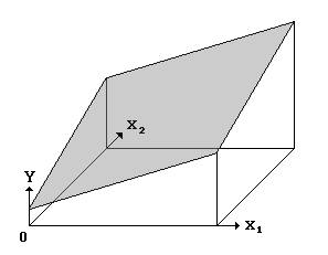
Figure 2: The Canonical Cusp Surface.

The cusp catastrophe model is a response surface that contains a smooth pleat, as in Figure 2. To obtain this amount of flexibility it is necessary to introduce 2v+2 additional degrees of freedom in the model. This is done by defining three "control factors," each a scalar-valued function of the vector X = (X₁, ..., X_v) of independent variables:

This prediction equation is a cubic polynomial in Y, which means that for each value of X there are either one or three predicted values of Y, as seen in Figure 2.

The individual effects of the factors A and B on Y can be seen in Figures 3a and 3b. For simplicity, it is assumed in these figures that C=0 and D=1. Note that the panels in these figures represent vertical slices cut through the canonical cusp surface (Figure 2). Figure 3a exhibits slices that are parallel to the A axis of Figure 2, while the slices depicted in Figure 3b are parallel to the B axis.

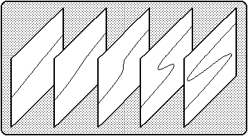
Figure 3a: The effect of A on Y, with B = (-5.0, -2.5, 0.0, +2.5, +5.0).

The individual effects of the factors A and B are depicted in Figures 3a and 3b as if they were independent, but according to the assumptions of the model both A and B depend on X. However, a comprehensive discussion of the effect each component of X on Y must be deferred until later.

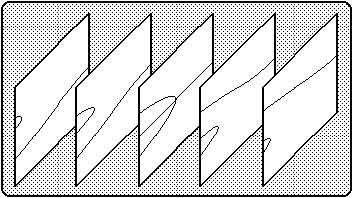
Figure 3b: The effect of B on Y, with A = (-3.0, -1.5, 0.0, 1.5, 3.0).

According to the terminology generally used in the literature on catastrophe theory, A and B are the socalled "normal" and "splitting" factors, respectively (the term "normal" is used simply because this factor is perpendicular, i.e. normal, to the splitting factor in the canonical representation of the control space). I recommend avoiding this terminology for two reasons: (a) to prevent confusion with the normal distribution, and (b) to emphasize the fact that the statistical model is not as flexible as the topological model. In this paper, A, B, and C will be called the asymmetry, bifurcation, and linear factors, respectively.

Those familiar with the literature on applications of catastrophe theory may wonder about the linear factor C and the coefficient D in the previous equation, since they are not ordinarily seen in the equations which define the canonical cusp catastrophe model. The usual equation for the canonical cusp surface, which in terms of our variables would be written as

The statistical catastrophe model defined by Equation 3 can be seen as a generalization of the regression model (Equation 1): the two models coincide if (1) A=0, (2) B=1/Var[U], and (3) D=0. When these conditions are satisfied the coefficients C_i of C are the same as the coefficients b_i of Equation 1. In fact, these are the initial values used by the maximum likelihood method when it begins its iterative search for the best fitting coefficients for the catastrophe model.

The statistical model based on Equation 3 is, like the regression model described by Equation 1, a static random model. It is useful to remember that the static catastrophe model is related to, and indeed derived from, a dynamic model. The (deterministic) dynamic cusp catastrophe model is described by a differential equation:

In this formulation a, b, and c are scalar-valued functions of the vector x, and d is a scalar. For each value of x this dynamical system has either one or three equilibria. These are the values of y for which dy/dt = 0. Thus the equilibria of the dynamical system correspond exactly to the predicted values of the static system. One could use the theory of stochastic difference equations to derive from Equation 5 a statistical model appropriate for nonlinear time series analysis, but that is a research topic that is inappropriate here (see Cobb & Zacks, 1988). The approach we take here assumes that a time series is not available, and that the data take the form of a random sample of statistically independent replicates of the system, observed at one single point in time. Thus we are considering the static random case. To complete the specification of the statistical model, it remains to specify the probability density function for the random variables in Equation 3.

Estimating the Parameters

Cusp Surface Analysis uses the method of maximum likelihood to estimate the parameters in Equations 2 and 3. The values of X are assumed to be fixed experimentally or measured without error. The conditional probability density function for Y given X is assumed to be the Type N3 density in the typology given in [Cobb, Koppstein, and Chen, 1983]. This PDF has either one mode or two modes separated by an antimode. These modes and antimodes are precisely the solutions to Equation 3. Therefore the predictions made by the cusp model are the modal values of the conditional density of Y given X. The antimode is an "antiprediction" — a value that is specifically identified as "not likely to be seen."

The differences and similarities between linear regression and Cusp Surface Analysis are worth careful examination. The conditional PDF of Y|X in linear regression is normal, i.e. Type N1 (an exponential of a quadratic), while the conditional PDF of Y|X in Cusp Surface Analysis is Type N3 (an exponential of a quartic). The predicted values in linear regression are the means of the conditional densities, which also happen to be modes, while in Cusp Surface Analysis the predicted values are modes (and the densities are frequently bimodal, yielding two predictions). Lastly, in linear regression the formulas for the sampling variance of the estimators are known exactly, while in Cusp Surface Analysis the corresponding formulas are approximations.

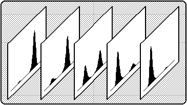
Figure 4a: The Type N3 PDF for the cusp catastrophe model,
with B = 4, C = 0, D = 1, and A = (1, .5, 0, -.5, -1).

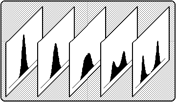
Figure 4b: The Type N3 PDF for the cusp catastrophe model,
with A = 0, C = 0, D = 1, and B = (-2, -1, 0, 1, 2).

The Cusp Surface Analysis program begins with the estimated coefficients of the linear regression model, and iterates towards the parameter vector that maximizes the likelihood of the cusp model given the observed data. The iterative scheme is a modified Newton-Raphson (NR) method. If the very first iteration yields a decrease in the the likelihood function, the program immediately halts with a message indicating that the linear model is preferable to any cusp model (this is a common occurrence). Upon successful convergence to a parameter vector that maximizes the likelihood function, the estimated coefficients of each factor are printed. If 20 iterations have been performed without convergence, the program prints out the results of the last iteration, but these results should be used for diagnostic purposes only.

The effect of A on Y is almost linear when B is negative (as in the leftmost panel of Figure 3a, for example). Thus when the empirical conditional distributions of Y|X are clearly unimodal there is a great deal of similarity between the effects of A and C. When this occurs, the estimators for the coefficients of these factors may be highly correlated (this occurs primarily in datasets with very few observations in the bimodal zone). In other words, the joint confidence region for pairs (A_i,C_i) of these estimated coefficients are highly elliptical. Stated in yet another way, when this occurs it means that A_i can be increased and C_i decreased, or vice versa, with very little effect on the likelihood function. To assist the user in diagnosing this condition, the program prints the estimated correlation matrix between the estimators for these coefficients. Correlations higher than about 0.9 indicate that these confidence regions are highly elliptical. If the NR algorithm halts before convergence (which could happen, for example, if the number of iterations reaches the cutoff value of 20), then this matrix cannot be estimated, and will contain only zeroes.

Testing the Model

The parameter estimates reported by the Cusp Surface Analysis program are useful for generating predictions, as described in the next section, but their values indicate nothing about their statistical significance. Therefore the program also reports an approximate t-statistic for each coefficient, with N–3v–3 degrees of freedom. These can be interpreted in the usual fashion: a magnitude in excess of the critical value indicates that the coefficient is significantly different from zero, at the specified significance level (remember that these t-statistics are only approximate). Of course, these statistics can also be misinterpreted in the usual ways too. For example, it is a mistake to pay attention to any of these values unless the overall model has passed all of its tests for acceptability. We now turn to these more general tests.

There is no single definitive statistical test for the acceptability of a catastrophe model. Part of the difficulty stems from the fact that a catastrophe model generally offers more than one predicted value for Y given X. This makes it difficult to find a tractable definition for prediction error, without which all goodness-of-fit measures that are based on the concept of prediction error (e.g. mean squared error) are nearly useless. Another part of the difficulty arises from the fact that the statistical model is not linear in its parameters. And finally, of course, it is scientifically unsound to base any definitive statement on the analysis of a single data set, no matter what its statistics show. Confirmation must always be sought in the independent replication of results. In spite of these difficulties and caveats however, there are a variety of ways in which a catastrophe model may be tested through statistical means.

Cusp Surface Analysis offers three separate tests to assist the user in evaluating the overall acceptability of the cusp catastrophe model. To confirm a cusp model all three tests should be passed.

The first test is based on a comparison of the likelihood of the cusp model with the likelihood of the linear model. The test statistic is asymptotically chi-square distributed, which means that as the sample size increases the distribution of the test statistic converges to the chi-square distribution. The degrees of freedom for this chi-square statistic is the difference in the degrees of freedom for the two models being compared, i.e. 2v+2. Sufficiently large values of this statistic indicate that the cusp model has a significantly greater likelihood than the linear model.

Even if the first test shows that Equation 3 is superior to Equation 1, the correct model may still not be the cusp catastrophe model. This can happen if the estimate for D is not significantly different from zero, which it must be for the right hand side of Equation 3 to be a cubic polynomial in Y. If D were zero the prediction equation for Y would read like this:

Y = C(X) – A(X)/B(X)

This may be an interesting relationship, but it is clearly not a catastrophe model, since for each value of X there is precisely one value of Y (unless B(X)=0, in which case Y is undefined). The second test for the adequacy of the cusp model is, therefore, a comparison of D with zero. As it turns out, D must be positive for a PDF of Type N3 to be defined at all. Thus the appropriate test is a one-tailed t-test, computed using the approximate standard error of D. The degrees of freedom for this test is the sample size less the remaining degrees of freedom of the cusp model after D has been fixed at zero, i.e. N–3v–3.

Even if the model passes both of the preceding tests, it can happen that the only coefficients of the factors A and B which are significantly different from zero are A₀ and B₀. When this happens it is fair to say that the PDF of Y is indeed Type N3, but that no control variables have been found which can cause this density to shift between bimodal and unimodal. In this case the response surface is flat, and the coefficients of C determine its slope. If the PDF is bimodal then there are two parallel response surfaces.

Lastly, it may happen that both of the above tests may yield positive results for the cusp model, implying that the cubic polynomial in Equation 3 fits well enough, at least in a technical sense, but none of the observed values for X lie in the bimodal zone! In this event the location of the bimodal zone is only known by extrapolation from the given data. Since extrapolation is notoriously unreliable in statistical work, it is reasonable to require that some observations of X lie within the bimodal zone, while others lie outside. To assist the user in perceiving the estimated distribution of the data within the plane spanned by the asymmetry and bifurcation factors, the Cusp Surface Analysis program shows this 2-dimensional distribution, with the bimodal zone highlighted. As a rule of thumb, it is desirable to have at least 10% of the observations fall within the bimodal zone. This constitutes the third test.

To summarize, the cusp catastrophe model may be said to describe the relationship between a dependent variable Y and and vector X of independent variables if all of these three conditions hold:

1. The chi-square test shows that the likelihood of the cusp model is significantly higher than that of the linear model.
2. The coefficient for the cubic term and at least one of the coefficients of the asymmetry and bifurcation factors are significantly different from zero.
3. At least 10% of the data points fall in the bimodal zone of the estimated model.

Making Predictions

In the literature on applications of catastrophe theory there are two distinct ways of calculating predicted values from a catastrophe model. In the Maxwell Convention the predicted value is the most likely value, i.e. the position of the highest mode of the probability density function. In the Delay Convention a mode is also the predicted value, but it is not necessarily the highest one. Instead, the predicted value is the mode that is located on the same side of the antimode as the observed value of the state variable Y. Thus the delay convention uses as its predicted value the equilibrium point towards which the equivalent dynamical system would have moved. This is the convention most commonly adopted in applications of catastrophe theory, but there are circumstances in which the Maxwell convention is the appropriate one.

The Cusp Surface Analysis program calculates the predictions made under each convention for each datum, and from these it derives a number of statistics and graphs to aid the user in evaluating the quality of the predictions made under each convention, as follows:

• Modes and Antimodes: This page shows a list of the first 100 data, together with their estimated factors and modes.
  
  
• Delay-R²: This statistic is simply the estimated value of the quantity

1 – (error variance) / var[Y] ,

in which the errors are based on predictions of the delay rule. Although it is analogous to the multiple-R² of regression analysis, there are several important differences which are discussed below.

• Maxwell-R²: This is the corresponding statistic for the predictions of the Maxwell rule.
  
  
• Error Histogram: This graph depicts the distribution of the errors made under the delay rule. Also provided on this page are the mean and standard deviation of this distribution. These statistics are also known as the bias and standard error of estimate, respectively, of the estimates.

In multiple linear regression the estimates obtained by minimizing the mean squared prediction error coincide with those obtained by maximizing the likelihood function. In Cusp Surface Analysis this is not the case, and therefore the maximum likelihood estimates maximize neither the Delay-R² nor the Maxwell-R². Further, neither of these statistics is even guarranteed to be positive! Negative values occur when the cusp model fits so wretchedly that its error variance actually exceeds the variance of Y.

Users of the Cusp Surface Analysis program are urged to try analyzing random data of various types to learn more about how the program works. One such exercise, for example, is to create a set of data that are uniformly distributed about a linear trend. In this case the analysis should yield the correct slopes in the linear factor and a positive bifurcation constant, indicating a model with two parallel prediction lines. Experimentation of this sort will also drive home the importance of having a sufficiently large sample size.

A particularly interesting experiment with the Cusp Surface Analysis program can be performed by generating data that fall exactly on the canonical cusp surface (i.e. which exactly satisfy Equation 3, with C=0). One would think that the analysis should reproduce the correct coefficients with no error, but this is not what happens. Recall that Equation 3 only describes the deterministic model, and makes no statement about the conditional distribution of the random variable Y. On the other hand, the likelihood method makes the further assumption that this conditional distribution has a particular form, examples of which are depicted in Figure 4. Notice that in Figure 4a, for example, the relative height of the two modes changes very rapidly as the asymmetry factor increases. If the conditional distribution of Y in the manufactured data set does not behave similarly, then the cusp surface program will not yield the correct estimates. In fact, the maximum likelihood method will find the coefficients which best reproduce the empirical conditional distribution of Y, since this is roughly what it means to maximize the likelihood of a model.

Each of the component variables of X contributes to each of the factors A, B, and C, and the effect of each factor on Y depends on the values of the other factors. Thus it is hard to visualize and understand the effect of any given variable. For this reason the Cusp Surface Analysis program displays a graph of the effect that each of the independent variables would have on Y if every other variable were fixed at its mean value. Each graph shows the solutions to the cubic polynomial equation

0 = (A₀+A_iX_i) + (B₀+B_iX_i)[Y – (C₀+C_iX_i)] - D[Y – (C₀+C_iX_i)]³

for a given i. The solutions are graphed for |Y| < 2.5 and |X| < 3.0, a region which includes all but a tiny fraction of the observed values of X and Y. Thus even when there are three solutions the graph may display only one or two, indicating that the others are far outside the range of commonly observed values.

As an example of such a graph, Figure 5 shows how the coefficient C in Equation 6 can affect the relationship between X and Y.

Notice how the number and location of the catastrophe points cannot change as C changes, even though the graph itself undergoes considerable deformation. This is a "fiber-preserving" transformation (here the transformation is just Y —> Y–CX).

Figure 5: The effect of X on Y in Equation 4.2, for C = (-.50, -.25, 0.0, .25, .50).
Note that the number and location of the catastrophe points does not depend on C.

Program Messages

There are several conditions that will cause the Cusp Surface Analysis Program to terminate prematurely. If any of these conditions occur then the printed coefficients must not be considered correct ? they are printed for diagnostic purposes only. In this section the various abnormal conditions are described and interpreted.

1. Iterations halted: cubic coefficient is vanishing. The starting value of the coefficient for the cubic term (D) is 0. If the first (or any later) iteration of the Newton-Raphson search for the optimal coefficients yields a negative value for D, then the program halts with this message because D<0 is incompatible with the stochastic model. The conclusion we draw from this condition is that the linear model is correct.
2. Iterations halted: det(Hessian) is negative. The Hessian matrix is the matrix of second partial derivatives of the log-likelihood function with respect to the model parameters. When the current parameter estimate is close to a local maximum or minimum of the log-likelihood function, the determinant of the Hessian will be positive. When the determinant is negative the shape of the function in the neighborhood of the current parameter estimate resembles a saddle. This indicates that the Newton-Raphson method is highly unlikely to achieve convergence. This condition seems to occur when the estimation method cannot easily distinguish between a linear model with an N1 (normal) or an N3 probability density function. In either case there is little or no bimodality in the data, so the cusp model is not offering anything special. The conclusion we draw from this condition is that the linear model is correct.
3. Iterations halted: likelihood is not increasing. Some pathology, possibly numerical, is affecting the Newton-Raphson method. No conclusion can be reliably drawn from this condition, other than that the method failed. The cusp model might or might not fit.
4. Iterations halted after 20 with no convergence. The Newton-Raphson method failed to converge after a reasonable number of iterations. No conclusion can be reliably drawn from this condition, other than that the method failed. The cusp model might or might not fit.

An Example

The following document shows a sample printout from the Cusp Surface Analysis Program. Further examples may be found in Stewart & Peregoy (1983). This file is in PDF format, which requires the Adobe Acrobat Reader to view.

Sample.pdf

Bibliography

Cobb, L., Koppstein, P., and Chen, N.H., "Estimation and moment recursion relations for multimodal exponential distributions." Journal of the American Statistical Association, 78, 124-130, 1983.

Cobb, L., "Statistical Catastrophe Theory." In The Encyclopedia of the Statistical Sciences, Vol. 8. Edited by N.L. Johnson and S. Kotz. New York: Wiley-Interscience, 1988.

Cobb, L. and Zacks, S., "Applications of catastrophe theory for statistical modelling in the biosciences." Journal of the American Statistical Association, 80, 793-802, 1985.

Cobb, L. and Zacks, S., "Nonlinear Time Series Analysis for Dynamical Systems of Catastrophe Type." In Nonlinear Time Series and Signal Processing. Edited by R. Mohler. New York: Springer-Verlag, 1988.

Stewart, I.N., and Peregoy, P., "Catastrophe theory modelling is psychology." Psychological Bulletin, 94, 336-362.

---

Copyright © 1985 by Loren Cobb.
Revised: April 1998.